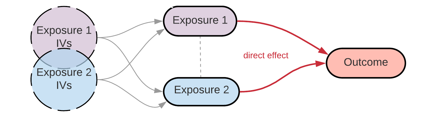
Setting up Multivariable Mendelian Randomization analysis in R
There are many tutorials and examples for performing a standard univariable Mendelian Randomization (MR) analysis using TwoSampleMR package. However, there is limited guidance available for setting up an efficient multivariable MR. It might be especially difficult to get started if you are using local data (i.e. not from MR-Base/OpenGWAS), or need to combine local and MR-base data, and also if you are looking to do your analysis with the newer multivariable MR package, MVMR.
In this blog post, I want to share my multivariable MR workflow. The workflow includes tidying up raw GWAS data (in my case, data from the IEU GWAS pipeline), doing the analysis first with the TwoSampleMR package, then converting the data into the format required for the MVMR package, and then repeating the analysis using it. Basically, this is the guide that I wish I had found a year ago when I first started doing MR analyses.
Disclaimer: I set up this workflow when I was working on my first ever MR project. It may not be the ultimate way to do it, but it worked well for me and I used it to reproduce the results from colleagues’ multivariable MR analyses. I’m still learning - if you know how to do it better, please share it.
Update (June 2021): Thank you Maria Sobczyk-Barad at MRC IEU for identifying the reason why TwoSampleMR and MVMR results don’t match perfectly and suggesting a solution. The code has been updated to use mv_harmonise_data in make_mvmr_input.
Quick summary of what this guide will show:
- how to prepare local GWAS summary statistics data files (i.e. raw output from a GWAS pipeline) for (any) MR analysis
- how to set up multivariable MR analysis with TwoSampleMR package on local files, or combine local files and MR-base traits in a single analysis
- how to create the input in the right format for use in the MVMR package
- the workflow will also work on >2 exposures
The blog post will focus on the analysis implementation and not the theoretical background or results interpretation.
Setup
In this example, I will perform multivariable MR on Adult BMI and Early life BMI as two exposures (from local text files generated with IEU GWAS pipeline from UK Biobank data) and breast cancer as the outcome (from MR-Base/OpenGWAS: ‘ieu-a-1126’, BCAC full sample).
For the analysis we need:
- exposure GWASs full summary statistics (tidy and formatted)
- exposure GWASs tophits (SNPs at p-value < 5e-8) (tidy and formatted)
- outcome GWAS full summary stats (will be accessed with TwoSampleMR from MR-Base, but also can use a local file)
library(readr)
library(vroom)
library(tidyr)
library(tibble)
library(dplyr)
library(TwoSampleMR)
library(MVMR)Load tophits data
NB these files have been pre-generated and tidied up, see the section at the end showing how they were created
# Load BMI exposures
adult_bmi_exp <- read_tsv(paste0(data_path, "adult_bmi_tophits.tsv"))
early_bmi_exp <- read_tsv(paste0(data_path, "early_bmi_adj_tophits.tsv"))Tophits in Adult BMI: 173
Tophits in Early BMI: 115The tophits files are in .exposure format (as used in TwoSampleMR)
glimpse(early_bmi_exp)
Rows: 115
Columns: 11
$ exposure <chr> "Early BMI", "Early BMI", "Early BMI", "Early B…
$ SNP <chr> "rs1546881", "rs212540", "rs582220", "rs2767486…
$ beta.exposure <dbl> -0.0125829, 0.0126875, -0.0114819, -0.0203200, …
$ se.exposure <dbl> 0.00223915, 0.00200119, 0.00195829, 0.00241081,…
$ effect_allele.exposure <chr> "T", "C", "A", "A", "G", "A", "T", "A", "C", "G…
$ other_allele.exposure <chr> "A", "T", "G", "G", "A", "G", "G", "G", "T", "A…
$ eaf.exposure <dbl> 0.627849, 0.392503, 0.433296, 0.798051, 0.48687…
$ pval.exposure <dbl> 1.9e-08, 2.3e-10, 4.5e-09, 3.5e-17, 5.6e-14, 2.…
$ mr_keep.exposure <lgl> TRUE, TRUE, TRUE, TRUE, TRUE, TRUE, TRUE, TRUE,…
$ pval_origin.exposure <chr> "reported", "reported", "reported", "reported",…
$ id.exposure <chr> "G4X7wF", "G4X7wF", "G4X7wF", "G4X7wF", "G4X7wF…Load full summary stats
NB these files have been pre-generated and tidied up, see the section at the end showing how they were created
# Load full GWAS for exposures
adult_bmi_gwas <- vroom(paste0(data_path, "adult_bmi_GWAS_tidy_outcome.txt.gz"))
early_bmi_gwas <- vroom(paste0(data_path, "early_bmi_adj_GWAS_tidy_outcome.txt.gz"))The full summary data for exposures is in .outcome format (as used in TwoSampleMR). This is required for harmonisation at a later stage.
Adult BMI full GWAS SNPs: 12298857
Early BMI full GWAS SNPs: 12298857glimpse(early_bmi_gwas)
Rows: 12,298,857
Columns: 11
$ SNP <chr> "rs367896724", "rs201106462", "rs575272151", "rs…
$ beta.outcome <dbl> 0.001015650, 0.002177780, 0.007636850, 0.0076368…
$ se.outcome <dbl> 0.00288045, 0.00296241, 0.00494634, 0.00494634, …
$ effect_allele.outcome <chr> "A", "T", "C", "C", "G", "T", "A", "G", "A", "T"…
$ other_allele.outcome <chr> "AC", "TA", "G", "G", "A", "G", "G", "C", "T", "…
$ eaf.outcome <dbl> 0.6016460, 0.6064280, 0.9141210, 0.9141210, 0.94…
$ pval.outcome <dbl> 0.720, 0.460, 0.120, 0.120, 0.120, 0.450, 0.450,…
$ outcome <chr> "Childhood BMI", "Childhood BMI", "Childhood BMI…
$ mr_keep.outcome <lgl> TRUE, TRUE, TRUE, TRUE, TRUE, TRUE, TRUE, TRUE, …
$ pval_origin.outcome <chr> "reported", "reported", "reported", "reported", …
$ id.outcome <chr> "1fWtbt", "1fWtbt", "1fWtbt", "1fWtbt", "1fWtbt"…Create list objects for the exposures
Next, we will create two list objects: tophits and full data of the exposures. These lists will be used as input for multivariable MR analysis in both TwoSampleMR and MVMR packages. If you have > 2 exposures to analyse, simply add the corresponding .exposure / .outcome data into the lists.
# create list objects for tophits and full gwas summary stats
tophits_list <- list(early_bmi_exp, adult_bmi_exp)
full_gwas_list <- list(early_bmi_gwas, adult_bmi_gwas)If you want to use one local exposure and another one from MR-Base, see supplementary section at end for details.
Multivariable MR with TwoSampleMR package
Multivariable MR with TwoSampleMR using MR-Base data is well-described in the original TwoSampleMR guide. Here I’ll be showing how to set up the first step of the analysis (i.e. extracting instrumental variables from the exposures) if your exposure data is local. NB please see the important note about this approach later.
I created a modified version of the original TwoSampleMR function mv_extract_exposures() for extracting instruments for multiple exposures: get_mv_exposures() uses as input the lists of tophits/full datathat we generated earlier and produces a data frame in the same format as the original mv_extract_exposures().
Using get_mv_exposures we create exposure_dat:
#Create exposure_dat, i.e. obtain instruments for each exposure (early BMI/adult BMI)
# (the function is defined later, remember to run it first)
exposure_dat <- get_mv_exposures(tophits_list, full_gwas_list)Next, we carry on with multivariable MR analysis as described in the TwoSampleMR guide:
#Next, extract those instruments/SNPs from the outcome (breast cancer MR-Base ID ieu-a-1126)
outcome_dat <- extract_outcome_data(snps = exposure_dat$SNP, outcomes = 'ieu-a-1126')
#Once the data has been obtained, harmonise so that exposure_dat and outcome_dat are on the same reference allele
mvdat <- mv_harmonise_data(exposure_dat, outcome_dat)
#Finally, perform the multivariable MR analysis
res_bmis <- mv_multiple(mvdat)
# Creating a tidy outcome
result_2smr <- res_bmis$result %>%
split_outcome() %>%
separate(outcome, "outcome", sep="[(]") %>%
mutate(outcome=stringr::str_trim(outcome))%>%
generate_odds_ratios() %>%
select(-id.exposure, -id.outcome) %>%
tidy_pvals()
result_2smr
exposure outcome nsnp b se pval lo_ci up_ci or or_lci95
1 Childhood BMI Breast cancer 82 -0.47 0.10 1.0e-06 -0.66 -0.28 0.62 0.52
2 Adult BMI Breast cancer 129 0.08 0.09 3.9e-01 -0.10 0.26 1.08 0.90
or_uci95
1 0.75
2 1.29Now let’s take a step back and inspect get_mv_exposures():
Please note: at the time of writing this blog post (March 2021), I discovered that a new function mv_extract_exposures_local() was added to TwoSampleMR guide in February 2021 (appeared in the codebase in May 2020). It is implemented in a very similar way with using lists, as my version get_mv_exposures() below. Therefore, I wanted to mention here that this is not an attempt to re-engineer the new existing TwoSampleMR’s function - I arrived at this solution independently when working on my first MR project in March-April 2020, and I have a dated Gitlab copy of this work from March 2020. I still wanted to write up this work in a blog post, as some parts of it might be useful to someone. I have tested the new function and confirmed that my solution produces the same results.
get_mv_exposures <- function(tophits_list, full_gwas_list) {
###
### This is a modified version of `mv_extract_exposures` function in TwoSampleMR package.
###
# Collapse list of exposures' tophits into a dataframe
exposures <- bind_rows(tophits_list)
# clump exposures: this will produce a list of instruments (shared and unique) of the given exposures
temp <- exposures
temp$id.exposure <- 1
temp <- clump_data(temp)
exposures <- filter(exposures, SNP %in% temp$SNP)
# subset full gwas summary stats of each exposure to the list of SNPs (instruments) produced above
for (i in 1:length(full_gwas_list)){
full_gwas_list[[i]] <- full_gwas_list[[i]] %>% filter(SNP %in% exposures$SNP)
}
# Collapse lists of subset gwas into a dataframe
d1 <- bind_rows(full_gwas_list) %>%
distinct()
### The logic of next steps is largely unchanged from the original function `mv_extract_exposures`
# get auto-generated ids
id_exposure <- unique(d1$id.outcome)
# convert first trait to exposure format -- exp1 is exposure
tmp_exposure <- d1 %>% filter(id.outcome == id_exposure[1]) %>% convert_outcome_to_exposure()
# keep other traits (n>=2) as outcome -- exp2+ are outcomes
tmp_outcome <- d1 %>% filter(id.outcome != id_exposure[1])
# Harmonise against the first trait
d <- harmonise_data(exposure_dat = tmp_exposure,
outcome_dat = tmp_outcome, action=2)
# Only keep SNPs that are present in all
snps_not_in_all <- d %>%
count(SNP) %>%
filter(n < length(tophits_list)-1) %>%
pull(SNP)
d <- filter(d, !SNP %in% snps_not_in_all)
# Subset and concat data
# for exp1 get exposure cols
dh1x <- d %>% filter(id.outcome == id.outcome[1]) %>%
select(SNP, contains("exposure"))
# for exp2 get outcome cols
dh2x <-d %>% select(SNP, contains("outcome"))
# rename outcome to exposure in these
names(dh2x) <- gsub("outcome", "exposure", names(dh2x) )
# join together (drop not needed cols)
exposure_dat <- bind_rows(dh1x, dh2x) %>%
select(-c("samplesize.exposure" ,"mr_keep.exposure", "pval_origin.exposure")) %>%
distinct()
return(exposure_dat)
}Multivariable MR with MVMR package
Next, we will create the input for multivariable MR analysis with the MVMR package. We can use the same tophits_list object and the exposure_dat data frame that were created as the inputs for the analysis with TwoSampleMR.
The required MVMR input format is well-described in the package vignette, and an example of what the data should look like is provided. However, when I was trying to create it for the first time, I found it quite challenging. So, after a few attempts and some guidance, I decided to automate it and created a function make_mvmr_input(). This function takes the same input as used by TwoSampleMR functions and generates the data in the format required for the MVMR function.
The function takes exposure_dat data frame and outcome.id.mrbase (dataset id in MR-Base) or outcome.data (if you want to use local data for the outcome - expects full GWAS data in .outcome format).
# create MVMR package input
# (the function is defined later, remember to run it first)
mvmr_input <- make_mvmr_input(exposure_dat, outcome.id.mrbase= 'ieu-a-1126')The function returns beta and se values for each exposure in mvmr_input$XGs and same for the outcome in mvmr_input$Y.
glimpse(mvmr_input$XGs)
Rows: 187
Columns: 5
$ SNP <chr> "rs10050620", "rs1013402", "rs10404726", "rs10510025", "rs10514…
$ betaX1 <dbl> 0.00968434, -0.02127110, 0.01384730, -0.01325810, -0.01372250, …
$ betaX2 <dbl> 0.015941500, -0.014079000, 0.008036340, 0.000228142, -0.0027969…
$ seX1 <dbl> 0.00210348, 0.00210760, 0.00197647, 0.00228816, 0.00196677, 0.0…
$ seX2 <dbl> 0.00206879, 0.00207208, 0.00194207, 0.00224989, 0.00193431, 0.0…
glimpse(mvmr_input$Y)
Rows: 187
Columns: 3
$ beta.outcome <dbl> -0.0114, 0.0045, 0.0152, -0.0010, -0.0100, 0.0076, 0.0053…
$ se.outcome <dbl> 0.0071, 0.0068, 0.0066, 0.0074, 0.0062, 0.0075, 0.0065, 0…
$ SNP <chr> "rs10050620", "rs1013402", "rs10404726", "rs10510025", "r…Next, we will select the required columns in mvmr_input when calling the format_mvmr() function from the MVMR package, which will further transform the data to work with the MVMR’s multivariable MR function.
# format data to be in MVMR package-compatible df
mvmr_out <- format_mvmr(BXGs = mvmr_input$XGs %>% select(contains("beta")), # exposure betas
BYG = mvmr_input$YG$beta.outcome, # outcome beta
seBXGs = mvmr_input$XGs %>% select(contains("se")), # exposure SEs
seBYG = mvmr_input$YG$se.outcome, # outcome SEs
RSID = mvmr_input$XGs$SNP) # SNPs
head(mvmr_out)
SNP betaYG sebetaYG betaX1 betaX2 sebetaX1 sebetaX2
1 rs10050620 -0.0114 0.0071 0.00968434 0.015941500 0.00210348 0.00206879
2 rs1013402 0.0045 0.0068 -0.02127110 -0.014079000 0.00210760 0.00207208
3 rs10404726 0.0152 0.0066 0.01384730 0.008036340 0.00197647 0.00194207
4 rs10510025 -0.0010 0.0074 -0.01325810 0.000228142 0.00228816 0.00224989
5 rs10514963 -0.0100 0.0062 -0.01372250 -0.002796960 0.00196677 0.00193431
6 rs10798139 0.0076 0.0075 -0.00875656 -0.013707400 0.00239406 0.00235527Now apply ivw_mvmr() MVMR’s multivariable MR function:
# estimate causal effects using method in MVMR package
mvmr_res <- ivw_mvmr(r_input=mvmr_out)
Multivariable MR
Estimate Std. Error t value Pr(>|t|)
exposure1 0.07809082 0.09081415 0.859897 3.909588e-01
exposure2 -0.47184441 0.09650650 -4.889250 2.188954e-06
Residual standard error: 1.711 on 185 degrees of freedomTidy up the output format:
result_mvmr <-
mvmr_res %>%
tidy_mvmr_output() %>%
mutate(exposure = mvmr_input$exposures,
outcome = 'Breast cancer') %>%
select(exposure, outcome, everything()) %>%
tidy_pvals()
result_mvmr
exposure outcome b se pval lo_ci up_ci or or_lci95
1 Adult BMI Breast cancer 0.08 0.09 3.9e-01 -0.10 0.26 1.08 0.90
2 Childhood BMI Breast cancer -0.47 0.10 2.2e-06 -0.66 -0.28 0.62 0.52
or_uci95
1 1.29
2 0.75Let’s take look closer at what is happening in the make_mvmr_input() function:
# function to convert 2SMR format into MVMR format
make_mvmr_input <- function(exposure_dat, outcome.id.mrbase=NULL, outcome.data=NULL){
# provide exposure_dat created in the same way as for TwoSampleMR
# also specify the outcome argument [only ONE!] (MR-base ID or full gwas data in .outcome format)
# extract SNPs for both exposures from outcome dataset
# (for the selected option mr.base or local outcome data)
if (!is.null(outcome.id.mrbase)) {
# if mrbase.id is provided
outcome_dat <- extract_outcome_data(snps = unique(exposure_dat$SNP),
outcomes = outcome.id.mrbase)
} else if (!is.null(outcome.data)){
# if outcome df is provided
outcome_dat <- outcome.data %>% filter(SNP %in% exposure_dat$SNP)
}
# harmonize datasets
exposure_dat <- exposure_dat %>% mutate(id.exposure = exposure)
outcome_harmonised <- mv_harmonise_data(exposure_dat, outcome_dat)
exposures_order <- colnames(outcome_harmonised$exposure_beta)
# Create variables for the analysis
### works for many exposures
no_exp = dim(outcome_harmonised$exposure_beta)[2] # count exposures
# add beta/se names
colnames(outcome_harmonised$exposure_beta) <- paste0("betaX", 1:no_exp)
colnames(outcome_harmonised$exposure_se) <- paste0("seX", 1:no_exp)
XGs <-left_join(as.data.frame(outcome_harmonised$exposure_beta) %>% rownames_to_column('SNP'),
as.data.frame(outcome_harmonised$exposure_se) %>%rownames_to_column('SNP'),
by = "SNP")
YG <- data.frame(beta.outcome = outcome_harmonised$outcome_beta,
se.outcome = outcome_harmonised$outcome_se) %>%
mutate(SNP = XGs$SNP)
return(list(YG = YG,
XGs = XGs,
exposures = exposures_order))
}Other functions used above:
tidy_pvals<-function(df){
# round up output values and keep p-vals in scientific notation
df %>%
mutate(pval= as.character(pval)) %>%
mutate_if(is.numeric, round, digits=2) %>%
mutate(pval=as.numeric(pval),
pval=scales::scientific(pval, digits = 2),
pval=as.numeric(pval))
}
tidy_mvmr_output <- function(mvmr_res) {
# tidy up MVMR returned output
mvmr_res %>%
as.data.frame() %>%
rownames_to_column("exposure") %>%
rename(b=Estimate,
se="Std. Error",
pval="Pr(>|t|)") %>%
select(-c(`t value`)) %>%
TwoSampleMR::generate_odds_ratios()
}Results comparison
Here is the side by side output comparison of two packages:
TwoSampleMR:
result_2smr %>% select(-nsnp)
exposure outcome b se pval lo_ci up_ci or or_lci95
1 Childhood BMI Breast cancer -0.47 0.10 1.0e-06 -0.66 -0.28 0.62 0.52
2 Adult BMI Breast cancer 0.08 0.09 3.9e-01 -0.10 0.26 1.08 0.90
or_uci95
1 0.75
2 1.29MVMR:
result_mvmr
exposure outcome b se pval lo_ci up_ci or or_lci95
1 Adult BMI Breast cancer 0.08 0.09 3.9e-01 -0.10 0.26 1.08 0.90
2 Childhood BMI Breast cancer -0.47 0.10 2.2e-06 -0.66 -0.28 0.62 0.52
or_uci95
1 1.29
2 0.75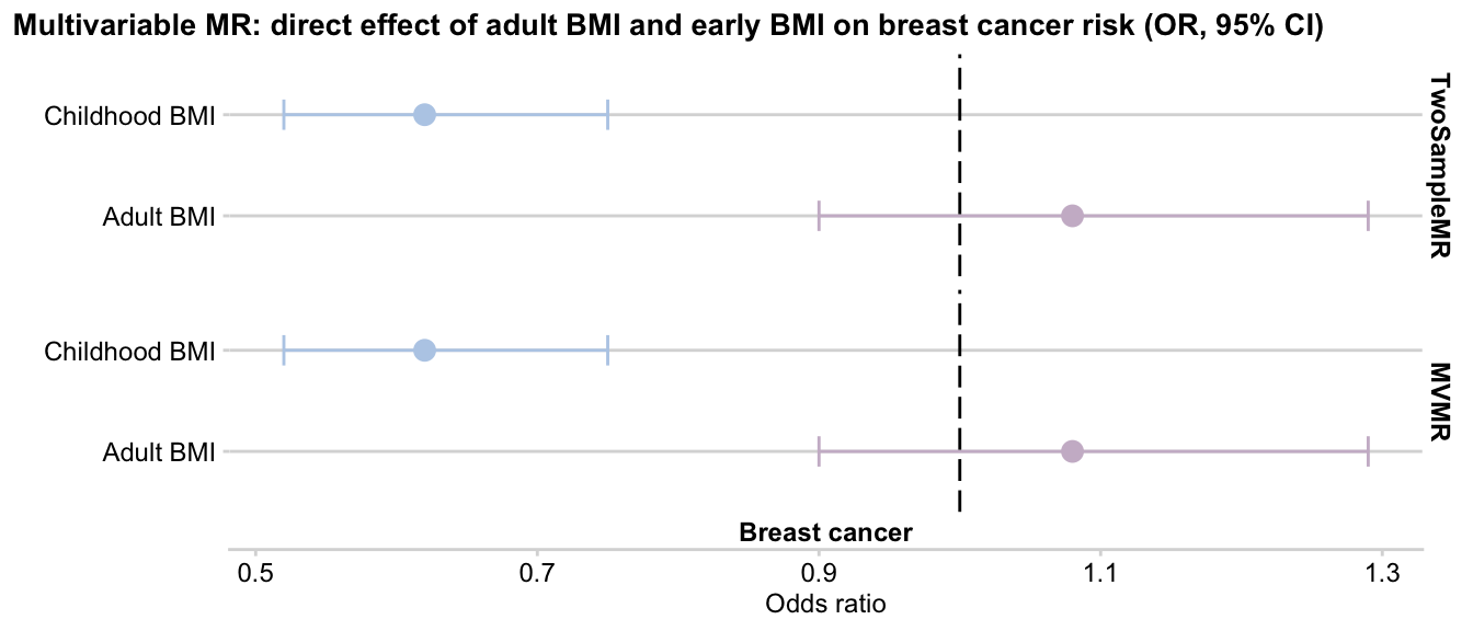
Supplementary: how to use exposures from mixed sources
Using one exposure from MR-base and another from local data is easy. Let’s say we want to keep Early life BMI as our first exposure (use the local data loaded above: early_bmi_exp and early_bmi_gwas) and the second exposure will be MR-Base trait ‘ieu-a-1095’, age at menarche.
# load instruments for MR-base trait
menarche_exp <- extract_instruments('ieu-a-1095')
## create a list object for tophits
tophits_list <- list(early_bmi_exp, menarche_exp)
# get all instruments from both exposures
tophits <- bind_rows(tophits_list) %>% pull(SNP)
# get all required SNPs from the 'full gwas' of MR-Base tarit in the .outcome format
menarche_gwas <- extract_outcome_data(snps = tophits, outcomes = 'ieu-a-1095')
## create a list object for full gwas of the traits
full_gwas_list <- list(early_bmi_gwas, menarche_gwas)Now tophits_list and full_gwas_list can be used in multivariable analysis as shown above.
(optional) Tidying up raw GWAS data
This section shows how I formatted raw data prior to the analysis and produced two files:
- tidy full GWAS file in TwoSampleMR
.outcomeformat - tidy tophits (i.e. SNPs at p-vale < 5e-8) file in TwoSampleMR
.exposureformat
# raw file location
raw_gwas_file <- paste0(data_path, 'adult_bmi_GWAS_raw_pipeline_output.txt.gz')
gwas_outcome_format <-
vroom(raw_gwas_file, # vroom is faster than fread!
# only read in columns that we need and
col_select = c("SNP","BETA","SE",
"ALLELE1","ALLELE0","A1FREQ",
"P_BOLT_LMM_INF")) %>%
# format data into the 'outcome' format right away
format_data(., type = "outcome",
snp_col = "SNP",
beta_col = "BETA",
se_col = "SE",
effect_allele_col = "ALLELE1",
other_allele_col = "ALLELE0",
eaf_col = "A1FREQ",
pval_col = "P_BOLT_LMM_INF") %>%
# store trait name in the data frame (this will make later analysis easier)
mutate(outcome = 'Adult BMI')
# save this tidy and formatted file so that it cam be used directly in MR analysis later
vroom_write(gwas_outcome_format, path = paste0(data_path,'adult_bmi_GWAS_tidy_outcome.txt.gz'))
# from the file that we read in, extract the tophits and save them in tophits file;
# this file will also be used directly in MR analysis later
tophits <-
gwas_outcome_format %>%
filter(pval.outcome < 5e-8) %>%
convert_outcome_to_exposure() %>%
clump_data(., clump_r2 = 0.001)
write_tsv(tophits, path = paste0(data_path, 'adult_bmi_tophits.tsv'))