Circular heatmaps of critical care bed occupancy rate in Bristol NHS Trusts, during a pre-COVID winter
This blogpost is a data story about critical care hospital occupancy rate in Bristol, in the winter of 2018-2019 (pre-COVID), for adults, children, and infants. It was originally submitted for a Christmas-themed data visualisation challenge at MRC-IEU programme 4 (challenge details).
- Dataset from NHS England: Winter SitRep: Acute Time series 3 December 2018 to 3 March 2019
- Visualisation tools: R packages circilize (https://github.com/jokergoo/circlize) and ComplexHeatmap (Bioconductor)
Background
The dataset contains critical care bed occupancy rates in all NHS Trusts across England from December 2018 to February 2019 (pre-COVID data). In my analysis/visualisation, I focus on Bristol data only.
Hospitals in Bristol are split between two NHS Trusts - North Bristol NHS Trust and University Hospitals Bristol and Weston NHS Foundation Trust, which cover the north and centre/south of the city, respectively. For context, below is the list of hospitals that belong to the two trusts [source]:
North Bristol NHS Trust (NBT) manages hospitals in the north of Bristol and South Gloucestershire.
- Southmead Hospital
- Cossham Memorial Hospital
- Frenchay Hospital
University Hospitals Bristol and Weston NHS Foundation Trust (UHB) manages hospitals in the centre and south of the city, and at Weston-super-Mare.
- Bristol Royal Infirmary (BRI)
- Bristol Heart Institute
- Bristol Haematology and Oncology Centre
- South Bristol Community Hospital
- Bristol Royal Hospital for Children
- St. Michael’s Hospital
- Bristol Eye Hospital
- University of Bristol Dental Hospital
Analysis
We are going to look at critical care bed occupancy rate for adults, children (<14 years), and infants (<6 months) in these two Bristol-based NHS Trusts (NBT & UHB), and visualise how occupancy rate changed over the winter months (especially during the holidays period! 🎅)
Load data
Reading the xls file and converting the data into the long format.
load_data <- function(file, sheet){
# function to load and tidy data from a specified sheet in the xls file
# read the dat in the specified sheet
dat<- read.xlsx(xlsxFile = file,
fillMergedCells = TRUE, colNames = FALSE,
sheet = sheet, rows = c(13:151))
# store NHS trust names and location separately
nhs_labels <- dat %>% select(region = X1, code = X3, Name= X4)
nhs_labels <- nhs_labels[5:nrow(nhs_labels),]
# store main data
data_values <- dat %>% select(X4:X277)
# vector of dates read in numerical format
dates_numerical <- data_values[2, 2:274]
# vector of value types
colnames_vector <- data_values[3, 2:274]
# create value type+date vector
new_names <-paste(colnames_vector, dates_numerical,sep='_')
# keep only values + add new colnames
data_values_only <- data_values[4:138,1:274]
colnames(data_values_only) <- c("Name", new_names )
# pivot data to long format; split type_date; convert date_numerical to Date; add NHS Trust labels
out <- data_values_only %>%
pivot_longer(!Name, names_to = "variable", values_to = "value") %>%
separate(col=variable, into=c("variable", "date"), sep = "_") %>%
mutate(date = openxlsx::convertToDate(date)) %>%
left_join(nhs_labels, by = "Name") %>%
arrange(region)
return(out)
}
dat_adult <- load_data(file = filename, sheet = "Adult critical care")
#preview
dat_adult %>% head %>% kable_it()| Name | variable | date | value | region | code |
|---|---|---|---|---|---|
| Barking, Havering and Redbridge University Hospitals NHS Trust | CC Adult Open | 2018-12-03 | 52 | London Commissioning Region | RF4 |
| Barking, Havering and Redbridge University Hospitals NHS Trust | CC Adult Occ | 2018-12-03 | 43 | London Commissioning Region | RF4 |
| Barking, Havering and Redbridge University Hospitals NHS Trust | Occupancy rate | 2018-12-03 | 0.82692307692307687 | London Commissioning Region | RF4 |
| Barking, Havering and Redbridge University Hospitals NHS Trust | CC Adult Open | 2018-12-04 | 52 | London Commissioning Region | RF4 |
| Barking, Havering and Redbridge University Hospitals NHS Trust | CC Adult Occ | 2018-12-04 | 46 | London Commissioning Region | RF4 |
| Barking, Havering and Redbridge University Hospitals NHS Trust | Occupancy rate | 2018-12-04 | 0.88461538461538458 | London Commissioning Region | RF4 |
Process data
Subsetting the data to Bristol NHS Trusts, and extracting bed occupancy rates for all winter day in the two NHS Trusts.
process_data <- function(data){
# function to subset data to Bristol/occupancy data only
# subset to Bristol
data_region <- data %>%
mutate(value=as.numeric(value)) %>%
filter(grepl("Bristol", Name)) %>%
mutate(abbr = case_when(Name == "University Hospitals Bristol NHS Foundation Trust" ~ "UHB",
Name == "North Bristol NHS Trust" ~"\nNBT"))
# keep only Occupancy data
data_region_occ <- data_region %>%
filter(grepl("Occupancy", variable))
# pivot data to wide format and keep winter only
data_region_occ_wide <- data_region_occ %>%
pivot_wider(id_cols=date, names_from = abbr, values_from = value, values_fill = NA) %>%
# extarct month from the date and create column with month name labels (set order with factor)
mutate(month = lubridate::month(date, label=T, abbr=F)) %>%
filter(month %in% c("December", "January" , "February")) %>%
mutate(month = factor(month, levels = c("December", "January" , "February"))) %>%
# create dat in 01-Dec format for the plot
mutate(DayDate=lubridate::day(date)) %>%
mutate(MonthDate=month(date, label=T)) %>%
unite(DayMonth, c("DayDate", "MonthDate"), sep = "-")
# keep month labels as a separate variable - will be used in viz for sectors
split <- data_region_occ_wide$month
# tidy the output
data_region_occ_wide<-
data_region_occ_wide %>%
column_to_rownames('DayMonth') %>%
select( "UHB", "\nNBT") # arrange in the order to appear on the plot
return(list(
full_bristol_data = data_region,
wide_data = data_region_occ_wide,
split = split
))
}
dat_adult_bristol <- process_data(dat_adult)
Warning in mask$eval_all_mutate(quo): NAs introduced by coercion
dat_adult_bristol$wide_data %>% head() %>% kable_it()| UHB | NBT | |
|---|---|---|
| 3-Dec | 0.8727273 | 0.6521739 |
| 4-Dec | 0.9090909 | 0.6739130 |
| 5-Dec | 0.9636364 | 0.7608696 |
| 6-Dec | 0.9818182 | 0.7391304 |
| 7-Dec | 0.9090909 | 0.7826087 |
| 8-Dec | 0.8181818 | 0.8043478 |
Visualise data (circular heatmap)
Here I define the plotting function -
plot_circular_heatmap <- function(df, title_prefix){
# function to draw a circular heatmap; inspired by -
# https://jokergoo.github.io/circlize_book/book/circos-heatmap.html
split <- df$split
df<- df$wide_data
# create color palette green-white-red (min to max occupancy)
vals <- c(df$`\nNBT`, df$`UHB`)
min <- round(min(vals[!is.na(vals)]),1)
mid = (1+min)/2
col_fun1 = colorRamp2(c(min, mid ,1), c("#0F3C28", "white", "#A7111C"))
# build plot by layers
circos.clear()
circos.par( gap.degree = c(5,5,20), start.degree = 150)
circos.heatmap(df, col = col_fun1, track.height = 0.4, rownames.side = "outside",
cluster=F, split = split, show.sector.labels = T,
bg.border = "grey", bg.lwd = 1, bg.lty = 1)
circos.track(track.index = get.current.track.index(), panel.fun = function(x, y) {
if(CELL_META$sector.numeric.index == 1) { # the last sector
cn = rev(colnames(df))
n = length(cn)
circos.text(x = rep(CELL_META$cell.xlim[2]+63, n) + convert_x(1, "mm"), # 63 is a magic number for moving track labels around the axis
y = 1:n - 3,
labels = cn,
cex = 0.8,
adj = c(0, 1),
facing = "inside")
}
}, bg.border = NA)
lgd = Legend(title = paste0(title_prefix,"\nbed occupancy"), col_fun = col_fun1)
grid.draw(lgd)
}Data story - critical care bed occupancy rate in Bristol NHS Trusts, during a pre-COVID winter
Adult critical care
The critical care occupancy rate (percentage of the available beds taken) is presented as a colour gradient heatmap: from green (beds available) to red (occupancy close to 100%). The data for NBT and UHB is shown as two separate tracks of the heatmap, going clockwise from December to February.
suppressMessages(
plot_circular_heatmap(df=dat_adult_bristol, "Adult critical care"))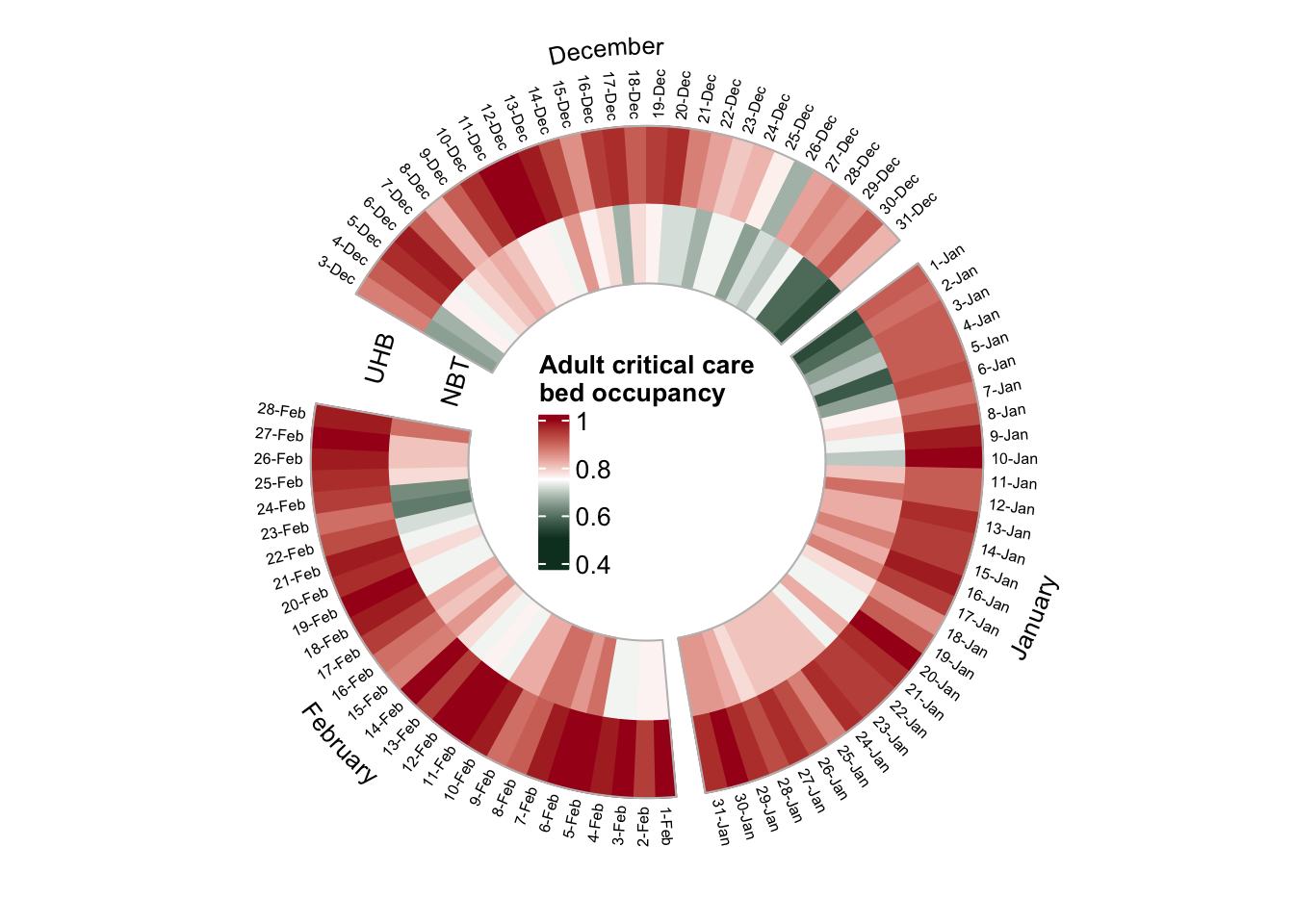
- UBH (n_beds=55) was very busy during the entire winter season (mean occupancy 93%)
- The only days with occupancy < 80% at UHB were Christmas and Boxing Days ☃️
- NBT (n_beds=46) was busy too (mean occupancy 76%), but there were fewer people in the critical care in NBT over the entire holiday season (~ 20-Dec to 6-Jan) ☃️)
# mean occupancy
round(colMeans(dat_adult_bristol$wide_data),2)
UHB \nNBT
0.93 0.76 # show the total number of available beds in each NHS Trust
dat_adult_bristol$full_bristol_data %>%
select(Name, abbr, variable, open_beds = value) %>%
mutate(abbr = gsub("\n", "", abbr)) %>%
filter(variable == "CC Adult Open") %>%
count(Name, abbr, open_beds) %>% filter(n>2) %>% select(-n) %>% kable_it()| Name | abbr | open_beds |
|---|---|---|
| North Bristol NHS Trust | NBT | 46 |
| University Hospitals Bristol NHS Foundation Trust | UHB | 55 |
Paediatric intensive care
Next, we look at bed occupancy rate in paediatric intensive care units, i.e. children (< 14 years)
# reusing the function defined for the adult critical care
dat_child <- load_data(file = filename, sheet = "Paediatric intensive care")
dat_child_bristol <- process_data(dat_child)
Warning in mask$eval_all_mutate(quo): NAs introduced by coercion
suppressMessages(
plot_circular_heatmap(df=dat_child_bristol, "Paedeatric \nintensive care"))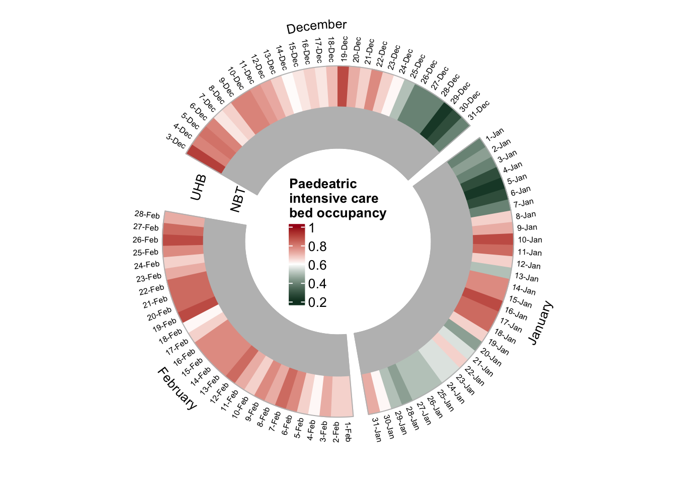
- Paediatric intensive care in Bristol is only available at UHB (likely at the Bristol Royal Hospital for Children), with mean occupancy 65%
- Therefore, no data is presented for NBT in the plot
- Bed occupancy was quite low in the paediatric intensive care between 25-Dec and 7-Jan: < 50% 🎁 ☃️ ☃️
# mean occupancy
round(colMeans(dat_child_bristol$wide_data),2)
UHB \nNBT
0.65 NA # show the total number of available beds* in each NHS Trust
dat_child_bristol$full_bristol_data %>%
select(Name, abbr, variable, open_beds = value) %>%
filter(variable == "Paed Int Care Open") %>%
mutate(abbr = gsub("\n", "", abbr)) %>%
count(Name, abbr, open_beds) %>% select(-n) %>% kable_it()| Name | abbr | open_beds |
|---|---|---|
| North Bristol NHS Trust | NBT | 0 |
| University Hospitals Bristol NHS Foundation Trust | UHB | 18 |
| University Hospitals Bristol NHS Foundation Trust | UHB | 33 |
*- The number of beds went from 33 to 18 on the 19th of December
Neonatal intensive care (NICU)
Finally, we look at occupancy rates in neonatal intensive care units (children at < 6 months)
dat_baby <- load_data(file = filename, sheet = "Neonatal intensive care ")
dat_baby_bristol <- process_data(dat_baby)
Warning in mask$eval_all_mutate(quo): NAs introduced by coercion
suppressMessages(
plot_circular_heatmap(df=dat_baby_bristol, "Neonatal \nintensive care "))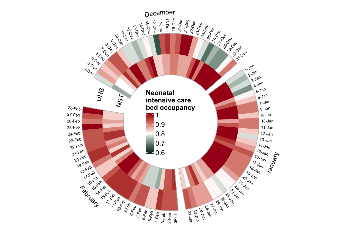
- NBT and UHB have a similar number of NICU beds (30/31)
- NBT was busier (92% mean occupancy), with ~100% beds taken from 23-Dec to 23-Jan
- At UHB a smaller number of beds were occupied from 24-Dec to 5-Jan ☃️
# mean occupancy
round(colMeans(dat_baby_bristol$wide_data),2)
UHB \nNBT
0.87 0.92 # show the total number of available beds in each NHS Trust
dat_baby_bristol$full_bristol_data %>%
select(Name, abbr, variable, open_beds = value) %>%
filter(variable == "Neo Int Care Open") %>%
mutate(abbr = gsub("\n", "", abbr)) %>%
count(Name, abbr, open_beds) %>% filter(n>10) %>% select(-n) %>% kable_it()| Name | abbr | open_beds |
|---|---|---|
| North Bristol NHS Trust | NBT | 30 |
| University Hospitals Bristol NHS Foundation Trust | UHB | 31 |
Final thoughts
- Critical care bed occupancy rate was high during the winter season pre-Covid
- High occupancy rate in neonatal intensive care may not be winter-season related
- Overall, there were less adults and children in critical care over the holiday season 🎁 🎅 🎁

All code is also available at https://github.com/mvab/winter_critical_care_bed_occupancy_NHS